The Diversifier Investors Thought They Already Had
Managed futures are moving into the mainstream. The next question is whether investors should buy the category — or the consensus behind it.
Daniel Li, PhD. Head of Index Research
In 2021, U.S.-listed managed futures ETFs held less than a billion dollars in combined assets. By May 2026, that number had reached roughly $7 billion, with the largest fund in the cohort tripling its asset base in roughly fourteen months. That kind of trajectory doesn’t happen because retail investors woke up one morning enthusiastic about commodity trading advisors. Something structural is pulling capital into a strategy that, for forty years, occupied a small, stable corner of institutional portfolios — typically around 3-5%.
The structural thing is that the bond side of the 60/40 stopped working, and nobody is sure when it will start again.
The diversifier that disappeared
In 2022 the Bloomberg Aggregate Bond Index lost roughly 13% while U.S. equities fell 19%. The 60/40 portfolio declined 17.5% — its worst calendar year since 1937 and its fourth-worst in two centuries. The decline itself wasn’t the most consequential part[1]. What mattered was that the 12-month rolling correlation between stocks and bonds approached +1.0, peaking near 0.80 in mid-2024. The mechanism that had carried balanced portfolios for forty years stopped functioning at exactly the moment investors needed it.
The longer-term picture, traced through the trailing three-year stock-bond correlation across both the Bloomberg Aggregate and the U.S. Government Index, makes the regime shift clearer than any single year of returns does:
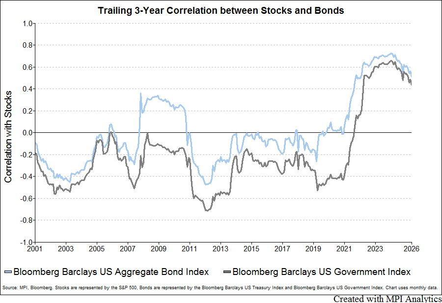
From 2001 through 2020, the correlation oscillated between -0.6 and 0.0, doing the diversifying work that the 60/40 was built on. From 2021 forward, it inverts, climbs above +0.6 by 2022, and only begins to fall in 2025. That’s the regime shift in one chart.
Defenders of the classic allocation point out, fairly, that this kind of positive correlation has happened before. Prior to 2000 it was the norm rather than the exception, and 2023’s snapback (the 60/40 returned 17.2%), combined with the gradual normalization of the correlation back toward 0.16 by late 2025, suggests the model is cyclical rather than broken. For an allocator sitting in 2026, though, with valuations elevated, inflation sticky, and central bank reaction functions still uncertain, eventually-correlated bonds don’t help with the year you’re actually in. The practical question is what to hold when bonds don’t diversify.
That is the gap retail flows are filling.
Where the capital is going
Retail investors didn’t just move to managed futures. They moved into a different version of managed futures than the one institutions have held for decades.
The split between channels is what tells the story. CTA and systematic-trading hedge fund AUM have been remarkably stable around the low-$300 billion range for a decade, with first-quarter 2026 net inflows of roughly $17.75 billion (about 6% growth). The retail-accessible wrapper category, by comparison, reached $6.9 billion in ETF assets as of May 11, 2026 — with $1.8 billion of year-to-date flows and $2.99 billion of one-year flows[2]. The institutional channel is larger by orders of magnitude, but the marginal demand is no longer arriving there.
The hedge fund channel has spent the last decade contending with a familiar set of pressures: fee compression, lengthening sales cycles, performance volatility tied to specific market regimes, and a generation of allocators who watched the post-GFC alpha narrative fail to deliver. Strategy AUM in that channel still dominates in absolute terms, but the marginal demand engine has migrated. The ETF and mutual fund versions of the same strategy, originally treated as retail novelties, are now where the asset growth is happening, where new product is being launched, and where the next cohort of allocators is forming its mental model of what managed futures is and what it does.
The ETF wrapper is the institutional product, repackaged for the channel where the demand is. If managed futures genuinely solved the post-2022 diversification puzzle, the rest of this would be a victory lap. It doesn’t, quite — and the reason is buried in the dispersion of returns within the category, which is where most of the practical risk for an allocator actually lives.
The dispersion problem hiding inside the headline
Take the cohort of the twenty largest institutional trend-followers in the world. In 2024, the average pairwise correlation between those twenty programs was 0.78. They were trading similar markets, on similar signals, in roughly similar regimes. And the range of annual returns across the constituents was nearly 15 percentage points. By the first four months of 2025, that range had widened to roughly 30 points, with category benchmarks down meaningfully year-to-date while individual short-term programs were posting gains.
Dispersion of this size exists in every active category. What makes it consequential here is the combination: a cohort trading similar markets on similar signals, producing similar correlations to equities, but delivering 15- to 30-point gaps in realized return[3].
The same dispersion shows up at the universe level, not only inside the elite cohort. Across the mutual fund and ETF managed futures universe over the four years from May 2022 through April 2026, the spread between the 5th and 95th percentile manager is roughly 14 points of annualized return, with the median sitting near zero and the worst-quartile drawdown reaching -33.8%:
| Statistic | Annual Return, % | Annual Stdev, % | Max Drawdown Return, % | Sharpe Ratio |
|---|---|---|---|---|
| Max | 12.95 | 23.22 | -6.56 | 0.58 |
| 5th percentile | 12.07 | 16.01 | -6.96 | 0.58 |
| 25th percentile | 4.76 | 13.03 | -11.98 | 0.10 |
| Median | 3.46 | 10.21 | -17.16 | -0.04 |
| 75th percentile | -0.58 | 8.05 | -21.45 | -0.35 |
| 95th percentile | -2.00 | 6.37 | -33.83 | -0.66 |
| Min | -3.04 | 5.82 | -34.44 | -1.02 |
| Note: Statistics are based on 34 funds (both mutual funds and ETFs) in the Morningstar’s U.S. Systematic Trend category over the May 2022–April 2026 period. Percentiles are calculated independently for each statistic across the universe over the period shown. For return, Sharpe and drawdowns, higher values indicate stronger outcomes; for standard deviation lower values indicate less volatility. | ||||
The category-level statistics — Sharpe ratio, max drawdown, correlation to equities — describe the asset class. They don’t describe what any individual investor ends up holding. An investor picking the right manager in 2024 captured the diversification benefit the strategy promises. An investor picking the wrong one, with identical due diligence and identical conviction in the asset class, ended up with a different outcome.
There’s a useful parallel in U.S. large-cap equities. Active managers in that category have, on average, delivered defensible returns for decades, and many continue to. Capturing the category-level outcome required selecting the right managers in advance, and most allocators found that difficult to do consistently. Index products emerged as a way to access the category for allocators who weren’t positioned to underwrite single-manager selection. Both approaches coexist today, and both have constituencies that buy them for sound reasons.
The consensus-of-PhDs idea
The methodological question is whether indexation is even possible for a strategy whose value proposition is, at first glance, the opposite of indexation. Trend-following is supposed to be skill. The whole pitch, since the 1980s, has been that systematic CTAs deserve their fees because their researchers — typically armies of physicists, statisticians, and quants — extract signal that the rest of the market can’t. Picking among them isn’t supposed to be replaceable by an index any more than active stock-picking was supposed to be replaceable by the S&P 500.
But the index investing argument never depended on active managers being unskilled. It depended on the observation that individually skilled managers, taken in aggregate, produce a different signal than any one of them produces alone. The skilled bets are correlated where the consensus is right and idiosyncratic where the consensus is uncertain. Aggregate those bets, let the idiosyncratic component cancel out, and what remains is the consensus exposure: the part of the strategy the cohort has, in aggregate, identified as the trend. The cancellation is the mechanism.
Apply that logic to the twenty largest systematic traders in the MPI Barclay Elite Systematic Traders Index, and the analytical claim becomes more honest about what aggregation does and doesn’t require. The dispersion within the institutional cohort reflects a mix of factors — concentrated bets on different parts of the trend signal, differences in implementation, and yes, varying degrees of skill across managers. Aggregating across the cohort doesn’t depend on uniform skill. It depends on the idiosyncratic component of each manager’s positioning — whether driven by edge, error, or implementation — partially canceling in aggregate, leaving the consensus signal as the residual.
The aggregate is smoother than any of its constituents. Once the idiosyncratic risk cancels, the residual signal is closer to what most allocators wanted from the strategy in the first place than any single-manager exposure could be.
How this looks in actual market stress is the more useful test. Across the five most consequential stress regimes since 2000 — the dot-com bubble, the Global Financial Crisis, the post-COVID drawdown, the 2022 inflation spike, and the present Iran War period — the consensus benchmark and the two traditional building blocks of the 60/40 behaved very differently:
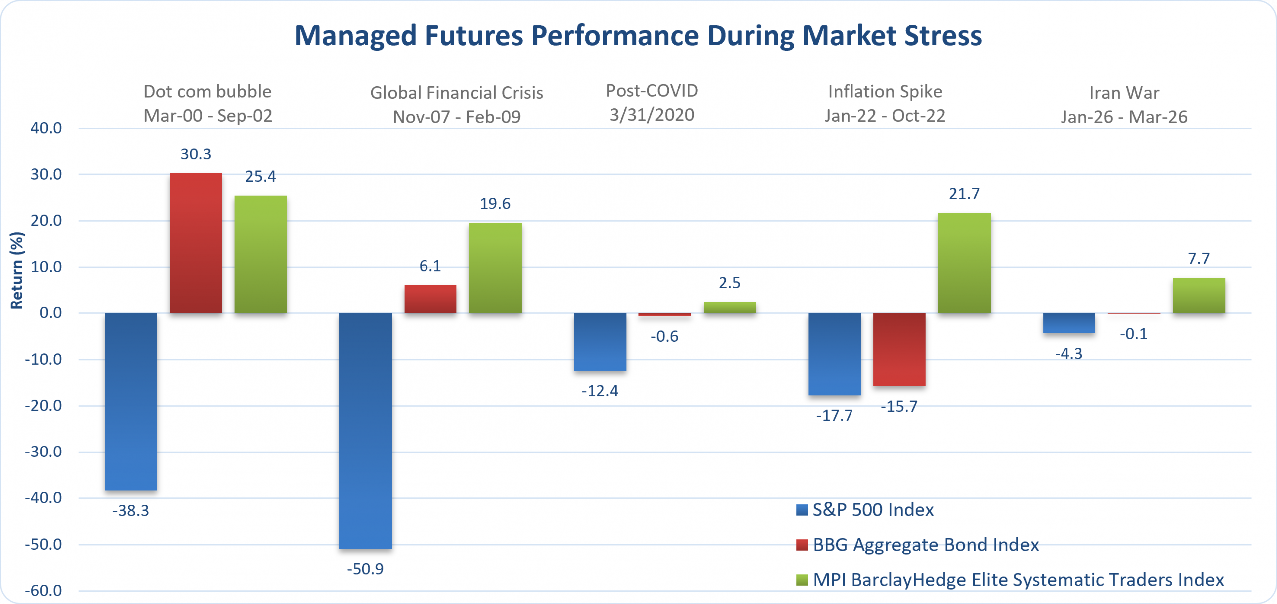
In four of the five regimes, the consensus benchmark either rose meaningfully (+25.4% in the dot-com bubble, +19.6% in the GFC, +21.7% during the 2022 inflation spike, +7.7% in the current Iran War period) or held within a single-digit drawdown while one of the two traditional building blocks was producing a double-digit loss. The exception is the post-COVID drawdown — a regime where rapid central bank intervention compressed trend signals across the cohort — and even there the consensus benchmark’s loss was small relative to either equities or bonds in their respective worst regimes.
The same pattern shows up in the long-run summary statistics:
| Jan-01 – Mar-26 | Annualized Return, % | Annualized StdDev, % | Sharpe Ratio | Max Drawdown Period | Max Drawdown Return, % | Correlation with MBEST, % |
|---|---|---|---|---|---|---|
| S&P 500 Index | 8.54 | 15.05 | 0.50 | Nov-07 – Feb-09 | -50.95 | -0.07 |
| BBG Aggregate Bond Index | 3.73 | 4.20 | 0.46 | Aug-20 – Oct-22 | -17.18 | 0.03 |
| MPI Barclay Elite Systematic Traders Index | 5.04 | 8.96 | 0.39 | Mar-04 – Jul-04 | -15.17 | 1.00 |
The Sharpe ratios across the three are within 0.11 of each other over a quarter-century. The consensus benchmark’s volatility sits between equities and bonds, its maximum drawdown is roughly a third of the S&P 500’s and close to bonds’, and its correlations to both are near zero.
MPI has been measuring this for eight years. Together with BarclayHedge, we developed the MPI Barclay Elite Systematic Traders Index[4] and launched its investable tracker to capture the average return of the twenty largest systematic traders. Our initial goal was to provide benchmarks for MPI’s institutional clients to assist in product selection and evaluation.
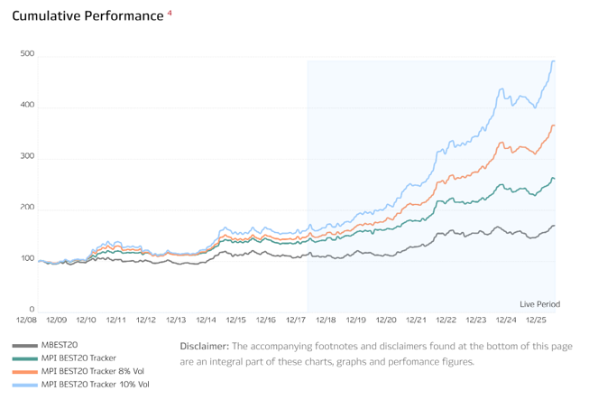
The short answer the data gives: the consensus exposure is meaningfully lower in volatility than any individual constituent, and it preserves the diversification properties — low correlation to equities, behavior across stress regimes — that institutional allocators were buying when they bought the category in the first place.
Placed against the Morningstar Managed Futures peer group on annual return, standard deviation, drawdown, and tracking error, the three vol-tier versions of the tracker cluster near the top quartile on return while sitting at or below the median on volatility and drawdown[5]:
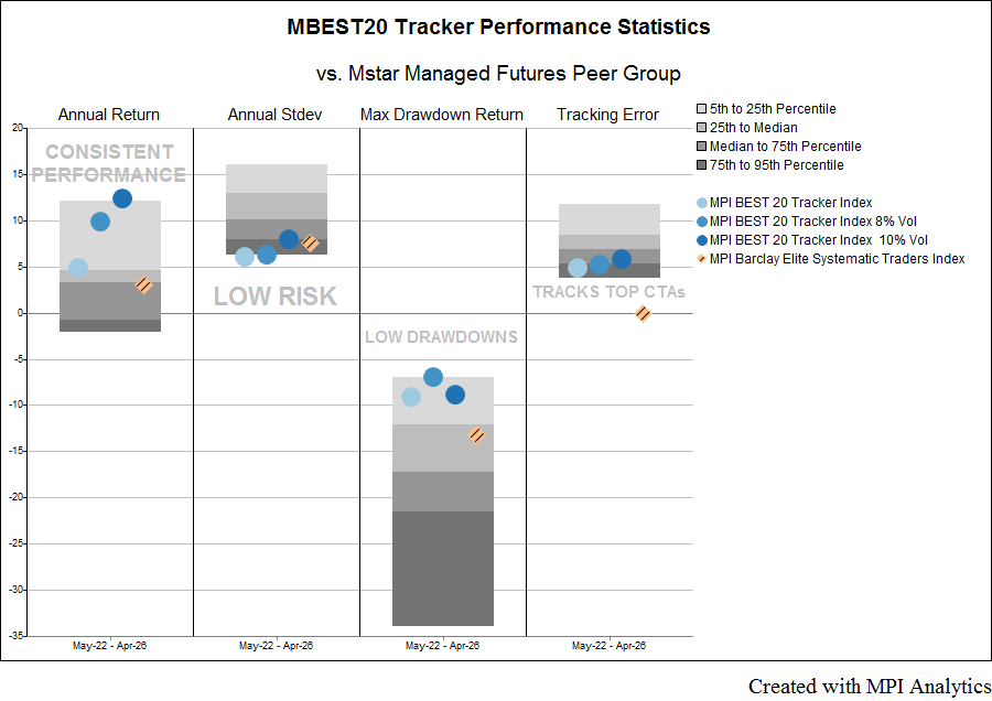 The label on the chart — “Consistent Performance / Low Risk / Low Drawdowns / Tracks Top CTAs” — is doing the summary work, but the substantive read is in the distance between the markers and the percentile bands.
What the data points to
Two characteristics show up consistently in the eight-year record. First, the consensus benchmark’s volatility profile sits closer to fixed income than to most alternative diversifiers, many of which carry more equity beta than their category labels suggest. Second, the correlation profile to equities stays near zero in the regimes where bonds correlate positively with stocks, which is the regime that made the diversification question urgent in the first place.
Saying that managed futures replaces bonds would be both inaccurate and bad sales practice; bonds carry duration risk and interest rate exposure that are useful in their own right, and a portfolio without them is a different portfolio. The narrower and more honest claim is that for an allocator looking at the post-2022 fixed income environment and asking where to put the diversification budget that bonds are no longer reliably earning, the consensus version of managed futures presents a profile that sits inside the conversation rather than outside it. That used to be a 5% conversation. The retail flows suggest it’s becoming a larger one.
The question MPI is watching
Whether managed futures belongs in broader portfolios is no longer a niche institutional question. Roughly $7 billion has already moved into U.S.-listed ETF wrappers, suggesting that allocators are increasingly looking for liquid, transparent ways to access the strategy. The harder question is not whether the category has a role, but how that exposure should be constructed — and whether investors are better served by selecting individual managers or by capturing the consensus signal behind the category.
That is the question MPI has been studying. Eight years of evidence on the consensus-of-PhDs approach suggest that index-based construction can help solve the category’s dispersion problem while preserving the diversification profile investors are seeking. As managed futures moves further into ETF and model-portfolio channels, construction may matter as much as allocation. If you’d like to see the underlying analysis, benchmark performance data, or discuss the methodology, please get in touch.
_________________________________________
[1] Stock-bond correlation figures sourced from BlackRock Investment Institute (December 2024) and Schroders historical analysis. The 2022 60/40 decline of 17.5% references Morgan Stanley Investment Management’s Big Picture: Return of the 60/40 and Morningstar’s 150-year stress test analysis.
[2] Industry AUM and ETF flow figures sourced from Morningstar’s Managed Futures: What to Know About This Strategy for ETFs (June 2024), AlphaSimplex’s The Rise of the Managed Futures ETF (April 2024), and ETF disclosure data through year-end 2025.
[3] Trend-following dispersion figures from Société Générale Prime Services & Clearing, Keeping up with the Trend-Followers, May 2025.
[4] The MPI Barclay Elite Systematic Traders Index (Bloomberg: MPBEST20) was developed in partnership with BarclayHedge in 2018 and is comprised of the twenty largest systematic traders reporting to the BarclayHedge database. The MPI BEST20 Tracker Index (Bloomberg: MBEST20T) is the investable daily tracker benchmark, available in standard, 8%, and 10% target volatility versions. The target-volatility versions are intended to facilitate comparisons across managed futures products with different volatility profiles.
[5] MPI Trackers are gross of fees and expenses
Technology Solutions
Trusted by